nForum
Not signed in
Want to take part in these discussions? Sign in if you have an account, or apply for one below
Site Tag Cloud
Vanilla 1.1.10 is a product of Lussumo. More Information: Documentation, Community Support.
If you want to take part in these discussions either sign in now (if you have an account), apply for one now (if you don't).
Atrium > Mathematics, Physics & Philosophy: Understanding Finite Limits
Bottom of Page1 to 59 of 59
-
- CommentRowNumber1.
- CommentAuthorEric
- CommentTimeJul 17th 2010
- (edited Jul 17th 2010)
In the paper
Jamie makes the following statement regarding cones over a diagram in a category whose objects are systems and morphisms are processes:
We could understand this physically as describing a simple sort of nondeterministic dynamics, where we evolve from an initial system at the bottom of the diagram to a final system towards the top, making a choice of process whenever more than one is available. Assuming for a moment that our systems are composed of sets of states, and our processes are functions, we can ask the following: are there any states of initial systems which will always transform into the same final state, regardless of the processes chosen? We could also take a more computational perspective, and regard the processes as constraints; an analogous question would then be to find the initial states which satisfy these constraints.
I really liked this statement. It made something click for me. When I asked Jamie where he obtained that intuition, he responded here:
However, I think that the moment this idea really clicked into place for me was when I read Joseph Goguen’s “A Categorical Manifesto”, where he describes limits in very similar terms.
So when I naturally chased up Goguen’s paper, we find:
The fourth dogma says:
A diagram in a category can be seen as a system of constraints, and then a limit of represents all possible solutions of the system.
In particular, if the diagram represents some physical (or conceptual) system, then the limit provides an object which (together with its projection morphisms) represents all possible behaviours of the system that are consistent with the given constraints. This intuition goes back to some work on General System Theory from 1969-74 [16,27], and has many applications in computing science.
There I got stuck. If someone with access to a good library might be able to somehow get me a copy of
[27] Joseph Goguen and Susanna Ginali, A categorical approach to general systems theory. In George Klir, editor, Applied General Systems Research, pages 257-270. Plenum, 1978.
I’d be forever grateful :)
Anyway, I think this intuition about limits is great and I hope to someday export some of it to the nLab, but I still don’t have a strong enough handle on it yet myself. Hence this thread :)
This is how I’m beginning to form my own intuition.
In a diagram, obviously not all diagrams need commute. This idea of “constraint” is pretty powerful (for pedestrians like me). If we think of objects as systems and morphisms as processes, then really a process/morphism is a constraint. A system that undergoes a process has satisfied the constraint .
If there are two constraints , then if following the process, a.k.a. satisfying the constraint, does not make you end up in the same state as following process , then that means that
does not satisfy both constraints
In other words, when category theorists say
“the diagram commutes”,
a physicist or engineer could read that as
“the initial system satisfies all constraints”.
In a general finite diagram, you can have all kinds of paths of processes and none of them need commute meaning that none of the given initial systems need satisfy all the given constraints.
A cone is a special initial system together with special processes that renders all the constraints of the original diagram to be satisfied. In other words,
A cone is a solution to all constraints of the diagram.
For example, with the two parallel constraints , we can say that does not satisfy both constraints simultaneously if the diagram does not commute.
However, a solution to these constraints would be a system together with a morphism such that
But also, for pedestrians like me, we can think of
as a “subsystem” of . So although did not satisfy the constraints, a solution to the constraints is a subsystem of .
For general finite limits, we just need to generalize this a bit, but I think this gets us at least 80% of the way there.
So now I think I understand morphisms as constraints and cones as solutions to constraints, but this is still only clear to me for parallel paths, i.e. equalizers. The only thing missing is how to incorporate products into this same picture and finally to see how any finite limit can be built from products and equalizers.
By the way, for the time being, I think I prefer to talk about cones as solutions until everything is perfectly clear because a limit is just a “special solution”, i.e. all cones are subsolutions of the limit.
-
- CommentRowNumber2.
- CommentAuthorTodd_Trimble
- CommentTimeJul 17th 2010
- (edited Jul 17th 2010)
Eric, at first the language you were using sounded mighty peculiar to me. Particularly, when I first read
If we think of objects as systems and morphisms as processes, then really a process/morphism is a constraint. A system that undergoes a process has satisfied the constraint .
I thought “uh-oh, this is really confused. What does it mean to say that a set has satisfied a function ?”. I still don’t think this is quite what you mean to say, but indeed there’s a way of thinking about this that leads more or less straight away to limits via products and equalizers.
In English, a constraint (e.g., a legal constraint) refers to a condition that has to be satisfied; in mathematics the constraint is quite often an equation that must be satisfied. In my mathematical education, I seem to have heard the word first used in reference to the method of Lagrange multipliers, where one is trying to optimize some function subject to a constraint of the form , a constant. That sort of thing.
Now a function acts on , but it doesn’t impose any kind of constraint on (elements of) . That is, you don’t need elements of to satisfy any particular condition in order to feed them into , not if the domain of is all of . So how is a constraint?
Answer: doesn’t impose a constraint on elements of , but it is a constraint on elements of the product . Namely, “a pair satisfies the constraint ” should mean it satisfies the condition . (If you think of a graph of a function as some subset of , then we just mean the point belongs to that subset.)
Similarly, we can view a diagram
as imposing a pair of constraints on elements , namely we must have both and . If you want, you can view this as a constraint on elements of , namely the imposition of the condition . Either way, we get a description of the equalizer as the set of all solutions to that pair of constraints: you could say
The equalizer is the set of all pairs such that and
or you could equally well say
The equalizer is the set of all such that
These descriptions are not literally the same as sets, but these sets are in bijection with (are isomorphic to) one another. In one direction, the bijection takes an element satisfying to the pair . In the other direction, it takes a pair satisfying and to the element . [Similarly, the set of satisfying is in bijection with the set .]
Anyway, any diagram can be similarly interpreted as imposing a system of constraints named by the morphisms that appear in the diagram, and the limit of the diagram is, as you say, the set of all solutions satisfying the system of constraints. Let’s try another: suppose we have the diagram
This time we see three objects, and the diagram is to be considered as a system of constraints on elements of the triple product . Namely, the constraints on are that and . The limit of this diagram, more familiarly the pullback of this diagram, can be described either as
The set of all such that and
or equivalently (up to isomorphism)
The set of all such that
and you should convince yourself of the easy exercise that these descriptions are indeed isomorphic to each other.
Having done this, there is no need to constrain ourselves (ha ha) any further: any diagram whatsoever can be similarly interpreted as a system of constraints. Constraints on what? On elements of the product of all objects appearing in the diagram.
So, how would this apply to products? A product of and is the limit of the diagram which looks like this:
There are no constraints there, since no arrows appear in this diagram! It’s an empty diagram of constraints. That’s fine: so we therefore don’t impose any constraints on elements , and the solution set is the full product , and that’s the limit. Just as we expect.
Do we dare now say how this leads to a description of limits via products and equalizers? I think we’re just about ready to do that. In rough form, what we want is to carve out the limit as solution set as some subset of the product
of all objects appearing in the diagram. (Officially, a diagram is some functor , so the index actually refers to and ranges over the objects of , so that is the value of the object under the functor .) The elements of this product are tuples
and then we wish to impose constraints on these tuples, all of which take the form . The which appear here are morphisms which arise by applying the functor to a morphism in the category (and of course there may be more than one such morphism between and , as we know from the example of equalizers).
Basically, what’s going to happen is this: we’re going to glom all the equational constraints (named or indexed by morphisms of ) together into one master equation. It’s going to look something like this: we’re going to take an equalizer of a diagram of the form
where I’m not going to say what those two parallel arrows are yet (because to lay it all out precisely is going to require some preface which I don’t feel like squeezing into this comment), but this should give you an idea of the basic shape of things to come. If you are daring, you can try to figure it all out, but let’s stop here and see if this comment is helpful.
-
- CommentRowNumber3.
- CommentAuthorEric
- CommentTimeJul 17th 2010
- (edited Jul 17th 2010)
Awesome. Totally awesome. Thank you Todd :)
I was pretty sure I was finally getting the concept when I wrote it, so when I saw your opening comments, I started panicking a little. “Ack! I can’t even get THIS right?!?” But you managed to figure out what I meant.
From a pedestrian perspective, I think it will help understand limits by thinking in terms of constraints. Thinking of morphisms as constraints was a critical step in my “Eureka!” process. Language matters. So yes, a morphism is conceptually a constraint, but I didn’t say it quite right. I like the way you said it (especially since it is correct :))
We want to think of a morphism/process as a constraint on the bare product , which itself is a cone/solution with no morphisms/constraints. That is the key piece of intuition that was right in front of me, but I missed it until you said it. Yes, this is making sense now :)
After all,
itself is a diagram and all diagrams are systems of constraints.
Ok. Yes, very helpful. Thanks you :)
Ok…
Was about to submit this, but I can’t leave a comment without pushing things a bit, usually until I make some mistake :)
What is the limit of the diagram
?
Would it be something like the “graph of a morphism” , then we can represent this as a subsystem of the full product via some kind of inclusion
Edit: Added a bit later…
This seems like a general concept, e.g. the pullback can (I think) be drawn similarly
-
- CommentRowNumber4.
- CommentAuthorTodd_Trimble
- CommentTimeJul 17th 2010
- (edited Jul 17th 2010)
Yes, is the limit of , but as I say somewhere in my comment, this is isomorphic to . If you were to stop a randomly chosen category theorist walking by and asked what is the limit of the diagram , he’d probably say . :-)
There is no harm in drawing those horizontal arrows to products, but after a while you’ll probably quit doing that because it’s redundant. When you draw the components of the cone for , you have a pair of morphisms , , and such a pair determines a unique morphism to the product, , which is the one you intend with the horizontal arrow.
Finally, a nitpick: I wouldn’t say “constraint on ”, but “constraint on elements of ”. Even better, if you’re talking about a general category, you say something like this: morphisms can be identified with morphisms obeying the following constraints: . (Notice that I have now switched from speaking of elements to speaking of morphisms . When making the bridge from element-based mathematics to morphism-based mathematics, it is helpful to view morphisms as “generalized elements” of type .)
-
- CommentRowNumber5.
- CommentAuthorMike Shulman
- CommentTimeJul 18th 2010
This is a very nice discussion and should be recorded somewhere. At the risk of confusing things further, I would like point out that when you start doing higher-dimensional limits, differences such as between “the set of pairs (a,b) such that f(a)=b and g(a)=b” and “the set of all a such that f(a)=g(a)” start to become more important. For instance, if A and B are categories and f and g are functors, then “the category of pairs (a,b) together with isomophisms and ” is not isomorphic to “the category of all together with an isomorphism ”, although they are equivalent. The first is the “pseudo-equalizer,” the second is the “iso-inserter.” And if you pass even further to the lax world, then you get “the category of pairs (a,b) together with mophisms and ” (a “lax equalizer”) and “the category of all together with a morphism ” (an “inserter”) which are no longer even equivalent.
For similar reasons, I think it is very good to think of the limit of a single arrow as the graph of , even though it is canonically isomorphic to A. If is a functor, then its pseudolimit is “the category of pairs (a,b) together with an isomorphism ,” and this is equivalent, but not isomorphic to, the category A. In fact, this pseudolimit is precisely the (iso)fibration part of the (acyclic cofibration,fibration) factorization of f in the (Lack) canonical model structure on Cat. If you don’t know what those words mean, don’t worry about it; I merely said it to make the point that the distinction between A and the pseudolimit of f matters. Even more interestingly, the lax limit of a functor is “the category of pairs (a,b) together with a morphism ”, and this, together with its projections to A and B, is one version of the graph of f. Another version of the graph of f is obtained from the colax limit, and the two versions of the cograph of a functor can similarly be obtained as lax and colax colimits.
-
- CommentRowNumber6.
- CommentAuthorIan_Durham
- CommentTimeJul 18th 2010
So, there is still something nagging at me that needs some clearing up. The wording of the following question may be a bit funky but hopefully someone will get what I’m trying to say. Cones obviously seem to be associated with, as Eric says, some kind of initial system. So there must be some relationship there to initial objects (or maybe some people call them 0-objects?). In any case, would there then be an analogous concept to cones that holds for terminal systems?
-
- CommentRowNumber7.
- CommentAuthorEric
- CommentTimeJul 18th 2010
Todd said:
Yes, is the limit of , but as I say somewhere in my comment, this is isomorphic to .
Initially I didn’t catch this, but looking back I now see your statement here:
[Similarly, the set of satisfying is in bijection with the set .]
But then Mike said:
For similar reasons, I think it is very good to think of the limit of a single arrow as the graph of , even though it is canonically isomorphic to A.
Very cool. So it seems that thinking of the limit of a single morphism as a graph carries over somewhat naturally to more generally contexts. I don’t recall ever seeing this stated before, but it is kind of neat and I’ll need to add it to Understanding Limits in Set. Thanks Mike :)
Ian asked:
Cones obviously seem to be associated with, as Eric says, some kind of initial system. So there must be some relationship there to initial objects (or maybe some people call them 0-objects?).
An initial object is an initial object of a category. A cone is an object that is appended to an existing diagram such that it becomes an initial object of that diagram. Diagrams do not need to be categories, so the ideas are related, but not exactly the same.
I recently learned a bit of trivial though that if a diagram already has an initial object, then that object is (isomorphic to) the limit. I thought of that when I saw Todd’s answer to my question about the limit of the simple diagram . Since is an initial object of the diagram, the limit is isomorphic to . But now after seeing Mike’s comment, I’m not sure how strongly I’d like to hold onto this bit of trivia. It may be fine for 1-categories but gets you in trouble later.
Then Ian asked
In any case, would there then be an analogous concept to cones that holds for terminal systems?
This is the yin-yang of category theory. Every statement has an opposite obtained by turning all morphisms around. What is initial in one diagram is terminal in the opposite diagram.
By the way, a zero object is an object that is both initial and terminal.
-
- CommentRowNumber8.
- CommentAuthorTodd_Trimble
- CommentTimeJul 18th 2010
- (edited Jul 18th 2010)
Mike: Yes, Eric has posed some very good questions and comments here, and it gives me a better idea how this stuff really ought to be taught. I’ve only taught category theory in the classroom once (it was an undergraduate class, but fairly good: Mark Weber was there and got his first taste of category theory from me!), so I’m really enjoying having this discussion. I certainly agree with your own comments.
Eric: All the ideas are in place, so I suppose we are now ready to tackle general limits via products and equalizers!
As a warm-up, let’s try the case of pullbacks first; I hope it will then be clear how to generalize. So, let’s review what we said about taking the limit of the diagram
in the category of sets and functions. This diagram is a functor where is the category with three objects and 2 nonidentity arrows:
We proceed in three steps:
Earlier we said that the limit of this diagram, the pullback, consists of all elements such that and . These equations “live” in (are valued in) , and we also have
where the refer to projection maps. Thus the first equation imposes the constraint
Similarly, the second imposes the constraint
Now comes a neat trick: we combine two equations into one by using products! The left-hand sides of equations (1) and (2) will be the two components , of a single map
and the right sides of (1) and (2) will be the two components , of a second map
The two equations (1) and (2) are then equivalent to the single equation . The limit of the diagram (here, the pullback) is the set of solutions to the system of equations (1), (2), or the set of solutions to the equation , in other words the equalizer of this pair of arrows. We have arrived at the products-and-equalizers presentation of the pullback as the equalizer of maps between products:
Finally, let us remark that while the discussion above was for the category , the same argument applies to any category. The elements , , should be replaced by “generalized elements” = morphisms , , ,
which are just the components of a cone with vertex . The triplet corresponds to a single map . The equations , means precisely that the map factors (uniquely) through the equalizer displayed above.
The construction for general limits is not too much of a stretch from here. Given a diagram , we think of each morphism in as tagging a constraint on (generalized) elements in the product
that must be satisfied in the limit. We again proceed in three parts:
If is a tuple of generalized elements, we want to impose, for each morphism , the constraint
With the aid of projection maps , this equation may be written
or, more simply, as morphisms from .
The maps on the left sides of these equations may be combined into a single map
and the maps on the right sides of these equations may be combined into a single map
To say that a collection are the components of a cone with vertex is to say that the tuple satisfies the entire -indexed system of constraints indicated above. This is true if and only if , which is true if and only if factors (uniquely) through the equalizer .
This proves that the equalizer
is a vertex of a universal cone (i.e., is the limit of the diagram ), whose cone components are
and this completes the description of general limits in terms of products and equalizers.
-
- CommentRowNumber9.
- CommentAuthorEric
- CommentTimeJul 18th 2010
Wow! Thanks Todd :)
I only have a moment here, but wanted to say that you have shown a neat way to take a diagram, express it as a bunch of constraints, and then code this in terms of products and equalizers.
But now I’m wondering…
Physicists and engineers deal with constraints all the time and few of them are aware of limits and cones in categories. So I wonder if a procedure similar to the one you outlined here could be used in reverse? Take a set of constraints arising from some engineering or physics problem and recast it as a diagram in some category. That would be cool.
Can anyone think of an example physical problem with constraints we could try to reverse engineer into a diagram in some category?
-
- CommentRowNumber10.
- CommentAuthorUrs
- CommentTimeJul 18th 2010
Can anyone think of an example physical problem with constraints we could try to reverse engineer into a diagram in some category?
In the simplest setup, think of a phase space with a constraint function on it. The constraint surface is the limit over
Now, this may not exist as a smooth manifold, but only as something more general. In fact, in BV-quantization or homological symplectic reduction, one realizes this as a limit in derived geometry, i.e. as a homotopy limit. (keyword: Koszul-resolution).
I’ll have to leave it at this hasty comment right now. Hopefully some other time I have the leisure to expand on this. We also still need to expand our entry BV-BRST formalism at some point…
-
- CommentRowNumber11.
- CommentAuthorEric
- CommentTimeJul 18th 2010
- (edited Jul 18th 2010)
Interesting. Thanks Urs. So if the limit does not exist as a smooth manifold, then you must be in a category other than that of smooth manifolds. Just out of curiosity, what category would you be working in for something like this? Are smooth spaces sufficiently general for this kind of example?
Edit: Just had a look at BV-BRST formalism. The answer to my question is probably there, but… gulp
-
- CommentRowNumber12.
- CommentAuthorUrs
- CommentTimeJul 18th 2010
- (edited Jul 18th 2010)
what category would you be working in for something like this?
derived smooth manifolds. Things that do not have just rings of smooth functions on them, but chain complexes of rings of smooth functions.
In BV-formalism, the components of these complexes of functions are known as the “antifields”.
Edit: Just had a look at BV-BRST formalism. The answer to my question is probably there, but… gulp
This is a stub entry not meant for public consumption. As I said, we still need to find time to work on it…
-
- CommentRowNumber13.
- CommentAuthorEric
- CommentTimeJul 19th 2010
derived smooth manifolds. Things that do not have just rings of smooth functions on them, but chain complexes of rings of smooth functions.
Ok. Although I won’t pretend to understand completely, the haze in my head was lifted a little bit. Thanks.
In fact, it seems you are directly using the concept of “oppositality” to define your category of spaces, i.e. as the opposite of .
By the way, my “gulp” was not meant as a criticism of the page, which looks really interesting to me, but rather an acknowledgment of my own personal limitations :)
-
- CommentRowNumber14.
- CommentAuthorIan_Durham
- CommentTimeJul 19th 2010
@Eric: Thanks for clearing up the distinction between initial objects in diagrams and categories - and the yin/yang of category theory. There is something quite beautiful about that. I need to do some thinking about how this relates to physical systems.
-
- CommentRowNumber15.
- CommentAuthorDavidRoberts
- CommentTimeJul 19th 2010
- (edited Jul 19th 2010)
The comment previously here was utter rubbish.
-
- CommentRowNumber16.
- CommentAuthorEric
- CommentTimeJul 19th 2010
- (edited Jul 19th 2010)
I thought the limit was the terminal object in the category of cones. Since any solution (cone) is a sub-solution of the general solution (limit) there is a map .
This also seems to be the way it is expressed in Section 3.1 of Basic Category Theory (unless I’m misinterpreting it).
PS: I like the above reference a lot too.
-
- CommentRowNumber17.
- CommentAuthorDavidRoberts
- CommentTimeJul 19th 2010
Whoops! I am a silly old duffer! Got a bit carried away there. I blame waking up at 5.30 this morning. Herm herm.
-
- CommentRowNumber18.
- CommentAuthorUrs
- CommentTimeJul 19th 2010
- (edited Jul 19th 2010)
Eric,
please never mind my BV comments, I didn’t want to distract from the very good discussion about basics of limits here, just wanted to indicate that the effort is not all wasted when it comes to serious applications in theoretical physics.
I am enjoying seeing you say sentences like
I thought the limit was the terminal object in the category of cones.
And, yes, that’s true.
-
- CommentRowNumber19.
- CommentAuthorEric
- CommentTimeJul 19th 2010
By the way, the type of examples I was looking for were more “physics 101” or “engineering 101” in nature. Googling leads to all kinds of interesting stuff:
- Principles of Constraint Systems and Constraint Solvers
- Irreducible System of Constraints for a General Polyhedron of Arrangements
- Numerical Solving of Geometric Constraints by Bisection: A Distributed Approach
- Two types of topological constraints in polymer networks
- Nonholonomic constraint: Mechanics of Manipulation
- Etc etc
The list goes on and on. I wonder how many of these “systems of constraints” can be represented as diagrams of some category. Then solutions to these systems of constraints would be cones/limits of the corresponding diagrams.
-
- CommentRowNumber20.
- CommentAuthorUrs
- CommentTimeJul 19th 2010
Well, every equation is an equalizer diagram, hence every equation in physics 101, say the “constraint”
is an equalizer diagram, hence every solutuion of it an element of the limit over that diagram.
So just looking at bare constraint equations won’t give much insight beyond the familiar fact that there are equations governing physics.
I’ll try to think of an example of limits in physics of the kind you might find useful…
-
- CommentRowNumber21.
- CommentAuthorEric
- CommentTimeJul 20th 2010
Yeah, as one type of example I was thinking about something like maybe an equilibrium mechanics problems,
-
- CommentRowNumber22.
- CommentAuthorIan_Durham
- CommentTimeJul 20th 2010
I think a more interesting physical application (just thinking off the top of my head) would be something involving an asymptotic approximation. I was thinking in terms of computational things originally, but not just quantum-related. I used to do a lot of fluid dynamical work and there are a lot of limit approximations in fluid problems.
-
- CommentRowNumber23.
- CommentAuthorEric
- CommentTimeJul 20th 2010
- (edited Jul 20th 2010)
Yep yep. Computational physics (or finance) is definitely a research direction to take this. My phd research was in computational electromagnetics and I’d love to relate this stuff to numerical solutions to complex systems some day. An interesting application for me (but doubtful to others) would be mathematical finance. As I mentioned, a limit as described by Jamie and Goguen resonates with “no arbitrage” pricing methods in finance. Basically, the idea there is the price of the security should be “fair” independent of any economic outcome (much as described in Jamies paper). So the “limit” is the “fair” price of a security.
This financial concept has direct connections to Feynman path integrals. For example:
The Path Integral Approach to Financial Modeling and Options Pricing
Abstract In this paper we review some applications of the path integral methodology of quantum mechanics to financial modeling and options pricing. A path integral is defined as a limit of the sequence of finite-dimensional integrals, in a much the same way as the Riemannian integral is defined as a limit of the sequence of finite sums. The risk-neutral valuation formula for path-dependent options contingent upon multiple underlying assets admits an elegant representation in terms of path integrals (Feynman–Kac formula). The path integral representation of transition probability density (Green’s function) explicitly satisfies the diffusion PDE. Gaussian path integrals admit a closed-form solution given by the Van Vleck formula. Analytical approximations are obtained by means of the semiclassical (moments) expansion. Difficult path integrals are computed by numerical procedures, such as Monte Carlo simulation or deterministic discretization schemes. Several examples of path-dependent options are treated to illustrate the theory (weighted Asian options, floating barrier options, and barrier options with ladder-like barriers).
-
- CommentRowNumber24.
- CommentAuthorUrs
- CommentTimeJul 20th 2010
a lot of limit approximations in fluid problems.
The notion of limit in the sense of category theory as discussed here is not the notion of limit in analysis.
-
- CommentRowNumber25.
- CommentAuthorIan_Durham
- CommentTimeJul 20th 2010
The notion of limit in the sense of category theory as discussed here is not the notion of limit in analysis.
Right, but I was thinking in terms of how Jamie described them in his paper - more in terms of systems and processes.
-
- CommentRowNumber26.
- CommentAuthorEric
- CommentTimeJul 22nd 2010
Looking at Todd’s comment #8 above, I see that I am confused about some notation. What is
? This would make a little more sense to me if it said
but I doubt that is what is meant.
-
- CommentRowNumber27.
- CommentAuthorDavidRoberts
- CommentTimeJul 22nd 2010
- (edited Jul 22nd 2010)
A quick example should clear this up: suppose we have a category with 4 objects and non-identity arrows , and for . Then
is the product of the factors (one for each ) (one for each ) (one for each ), and (one for each identity arrow).
More generally there is a factor for each arrow of , and the factor itself is given by the value of the functor on the codomain of the arrow indexing that factor.
-
- CommentRowNumber28.
- CommentAuthorTodd_Trimble
- CommentTimeJul 22nd 2010
Eric, that product on the right needs to be an object, so we take a product of objects (not of morphisms ). I definitely had it the way it’s intended.
David is correct in what he wrote. If it helps notationally, we could also say that the limit is the equalizer of two parallel maps between the following two objects:
Just remember that a map to a product is tantamount to a collection of maps, one for each factor of the product. What maps? The ones you get by projecting down to each factor. Here it means that for each , the two maps displayed above project down to two maps to :
In this way we get a pair of maps from to for each , and the equalizer we constructed above will simultaneously equalize every such pair.
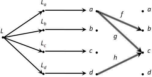
Here, let’s try another example. Suppose we want to apply this recipe to compute a limit of a diagram of shape
where as usual I am suppressing identity arrows so that there are four nonidentity arrows and five identity arrows, nine in all. A diagram of this shape in a category is a functor . What the equalizer of the diagram we are considering is doing is taking the set of solutions to a system which involves nine equations, one for each arrow in . For example, one of these equational constraints will correspond to the arrow , and it will look like this:
All this is saying is that we are putting the following constraint on a 5-tuple of :
You have similar equational constraints for each of the nine arrows of , and thus the limit is supposed to be the set of solutions to a system of equations
except what we did is combine nine equations into just one equation between elements of the product on the right:
and this is precisely what that big equalizer is set up to do: give the set of solutions to that single master equation.
-
- CommentRowNumber29.
- CommentAuthorEric
- CommentTimeJul 22nd 2010
- (edited Jul 22nd 2010)
If it helps notationally, we could also say that the limit is the equalizer of two parallel maps between the following two objects:
Just a quick note. Yes, this notation helps a lot. Thanks.
Edit: Actually staring at this helps a whole lot. This pretty much tells the whole story. Cool. I think I got it.
-
- CommentRowNumber30.
- CommentAuthorEric
- CommentTimeJul 22nd 2010
It is probably redundant, but in principle, could you write this as
?
-
- CommentRowNumber31.
- CommentAuthorEric
- CommentTimeJul 22nd 2010
Actually, I like writing it this way. It is an example of “extruding” a diagram. In other word, it is as though you make two copies of the set (since our diagrams are finite) of objects and pull the morphisms of the diagram so they extend from the domain in one copy to the codomain of the other copy. Any parallel morphisms are “equalized”.
I think this is optimally intuitive if not optimal in products :)
I’ll draw some diagrams when I find a moment.
-
- CommentRowNumber32.
- CommentAuthorDavidRoberts
- CommentTimeJul 22nd 2010
- (edited Jul 22nd 2010)
could you write this as $$ ?
no, because you have too many factors in the left product. Try my example above and see what you get for both versions.
-
- CommentRowNumber33.
- CommentAuthorEric
- CommentTimeJul 22nd 2010
Right right. I need to convert the picture in my head into the correct words. I think the picture is right. I think…
-
- CommentRowNumber34.
- CommentAuthorEric
- CommentTimeJul 22nd 2010
- (edited Jul 22nd 2010)
I worked out David’s example with some pictures of what I had in mind at:
Understanding Finite Limits (ericforgy)
The basic idea is to first “extrude” the diagram, i.e. make two copies of the set of objects and extend the morphisms from the domain in the first copy to the codomain in the second.
Then consider each subdiagram separately whose “leafs” are the individual objects.
The sublimit of this subdiagram is the object that equalizes all the parallel morphisms starting at that object simultaneously.
Then you repeat this and find the sublimits for each object of the original diagram.
The limit of the original diagram (I think!) is the product of these sublimits.
The punchline is the diagram
Have I gone completely off the deep end? Is there any truth to this?
It would be neat if a finite limit could be written as a product of sublimits/equalizers like this.
-
- CommentRowNumber35.
- CommentAuthorEric
- CommentTimeJul 23rd 2010
- (edited Jul 23rd 2010)
As I run out to catch a train…
Sorry. I see this is still not quite right. The final step needs to be an equalizer.
Just a note: I really really do appreciate all the help everyone gives me here. By trying to draw this procedure you’ve outlined, I am not trying to be fancy or cute. I have said before, but it is worth repeating now and then when the issue arises. I need to “see” it visually before I can learn it. I’m not exaggerating when I say that. So, I’m simply trying to draw a picture of what has been explained to me so far. My failure is just that, my failure. Any difference between what I described here and what has been explained is simply a matter of me not quite being able to understand it yet.
-
- CommentRowNumber36.
- CommentAuthorIan_Durham
- CommentTimeJul 24th 2010
I’m still on vacation, but I sketched out a rough diagram of a finite limit - sort of a “back of a napkin” kind of thing. I’m sure it’s not notationally correct, but I think it gets the basic idea across. I just don’t think it will work well in an SVG diagram. I’ll try to jot it down tonight and post it to see if I have the right idea or if I’m just delusional again.
-
- CommentRowNumber37.
- CommentAuthorEric
- CommentTimeJul 24th 2010
- (edited Jul 24th 2010)
Hey Ian,
Good luck with that :)
One piece of advice. Before you post your diagram, in order to save yourself the embarrassment I experienced above, you should check some things. You should check the following:
- The empty diagram
- A diagram with one object and no non-identity morphisms
- A diagram with one object and one non-identity morphism
- A diagram with two objects and no non-identity morphisms
- A diagram with two objects and one non-identity morphism between them
- A diagram with two objects and two parallel morphisms between them
- A diagram with three objects and two non-identity
I think my drawing above satisfies everything but the last item. I should have checked that last one before posting it.
I think I understand the concept, but available time is currently the only barrier keeping me from writing it down properly. Two non-equal parallel morphisms form a simple diagram that does not commute. The equalizer makes the simple diagram commute.
A more general limit (or at least a cone) can be thought of as a “commutizer”. It forces all parallel paths in the finite diagram to commute.
The thing I missed above is that although does not form any parallel paths in the original diagram, it does once you add the limit object and its components.
-
- CommentRowNumber38.
- CommentAuthorIan_Durham
- CommentTimeJul 24th 2010
Eric,
Maybe I’ll e-mail it to you to save myself the embarrassment. ;)
-
- CommentRowNumber39.
- CommentAuthorEric
- CommentTimeJul 24th 2010
Sure. Feel free :) Or we can work it out together here:
Understanding Finite Limits (ericforgy)
before sharing with the rest of the world.
-
- CommentRowNumber40.
- CommentAuthorIan_Durham
- CommentTimeJul 25th 2010
- (edited Jul 25th 2010)
Just uploaded my attempt at graphically understanding limits (in query box at bottom of page). -
- CommentRowNumber41.
- CommentAuthorDavidRoberts
- CommentTimeJul 26th 2010
Sorry, Ian, it doesn’t seem to have worked.
-
- CommentRowNumber42.
- CommentAuthorIan_Durham
- CommentTimeJul 26th 2010
Sorry, Ian, it doesn’t seem to have worked.
My upload or my attempt at understanding limits? :-)
-
- CommentRowNumber43.
- CommentAuthorDavidRoberts
- CommentTimeJul 26th 2010
- (edited Jul 26th 2010)
My mistake. I thought the upload hadn’t worked, but it has. Looking at it, I’m not sure what the diagram is supposed to indicate. What the colours signify isn’t obvious. Also, what it the shape of the diagram of which you are taking the limit?
-
- CommentRowNumber44.
- CommentAuthorEric
- CommentTimeJul 26th 2010
I’m not having any luck seeing the image.
-
- CommentRowNumber45.
- CommentAuthorDavidRoberts
- CommentTimeJul 26th 2010
When I clicked on the question mark after the tiff file name it downloaded fine. I’m not sure why the link displays like that - a question for our host perhaps.
-
- CommentRowNumber46.
- CommentAuthorIan_Durham
- CommentTimeJul 26th 2010
- (edited Jul 26th 2010)
Well, the colors don’t necessarily represent anything other than to make it clearer in my mind what was what.
I’m a doofus. I forgot to mention that this diagram is supposed to represent what is described in the first (full) paragraph on p.7 of Jamie’s paper.
-
- CommentRowNumber47.
- CommentAuthorEric
- CommentTimeJul 26th 2010
- (edited Jul 26th 2010)
Ian, if you email me the .tiff, I can make sure it displays properly. Now, it is completely gone :)

Images are a little tricky on the nLab.

Edit: Nevermind. I converted it to jpg and it is working fine now.
-
- CommentRowNumber48.
- CommentAuthorEric
- CommentTimeJul 26th 2010
- (edited Jul 26th 2010)
Have no time, but a quick comment.
Ian, aside from and , which should probably be and , this looks encouraging. It seems there is a good chance you understand the basic definition of limit.
Now to see if you understand what it means.
The cone you drew implies a specific equation. What is that equation? I’m talking only about the one (sub) cone you drew. What is the equation corresponding to that?
-
- CommentRowNumber49.
- CommentAuthorIan_Durham
- CommentTimeJul 28th 2010
Sorry, been insanely busy (with something you may actually be interested in with your dual background in E&M and finance, but I’ll save that for a personal e-mail).
Anyway, do you mean what is the equation that corresponds to the cone (and its corresponding cone map ?
-
- CommentRowNumber50.
- CommentAuthorIan_Durham
- CommentTimeJul 30th 2010
- (edited Jul 30th 2010)
So, in case that was what you were looking for, is what you’re asking for the following?
-
- CommentRowNumber51.
- CommentAuthorEric
- CommentTimeJul 30th 2010
Yep yep, except it is . I’ll assume a typo on the order and I took the liberty of replacing with :)
Now, what if there was a morphism . It’s cone enforces another similar equation.
Put the two cones together, they imply another equation. What is that other equation?
Finally, stick in another morphism . Its cone enforces another equation.
All of these little equations end up enforcing a relation between , , and . What is that relation?
-
- CommentRowNumber52.
- CommentAuthorIan_Durham
- CommentTimeJul 31st 2010
Right, so yes, the in the diagram and thus my equation should have been an . Regarding the order, it was less a regular typo than one of those things that’s probably related to mild dyslexia, i.e. I know it should be the other way but always seem to write it the wrong way for some reason.
Anyway, so the morphism implies the equation . Put the two together and you should get . The last morphism implies . This should imply that .
This stuff seems like it would be quite useful for circuit analysis, by the way.
-
- CommentRowNumber53.
- CommentAuthorEric
- CommentTimeAug 1st 2010
Hey Ian,
Welcome back :)
Yeah, the point was that when you glue commuting cones together, the result is a commuting cone. When two paths of commuting cones begin and end at the same objects, i.e. when they are parallel, the paths will commute. This is the reason I’ve personally adopted the name “commutizer” for the limit of a finite diagram :) All the little commuting cones force all diagrams in the original diagram to commute. It does a little more than that too. It forces paths in the original diagram that merely end at the same point to commute, because all paths in the limit share the same ultimate start point, i.e. the limit object itself.
By the way, it should be , but it seems like you go the idea.
I’ll think about circuits. I know John was spending some time on them recently in his TWFs, but I don’t remember if he was looking at limits of circuit diagrams interpreted category theoretically.
-
- CommentRowNumber54.
- CommentAuthorIan_Durham
- CommentTimeAug 1st 2010
Hey Eric,
One quick question so that I can really test the depth of my understanding here. I obviously know what is usually meant by ’commuting’ and think I understand the category theoretic use of the term, but it seems like in category theory there’s some kind of deeper je ne c’est qua at work here. To me, deep means simple. So, in the simplest way you can think, can you describe what you mean when you say all the diagrams commute?
Regarding circuits, I am particularly interested in this because I’m presently exploring relations between quantum circuits (i.e. those used in quantum information and computation) and classical electromagnetic circuits. In essence, I’m looking for some kind of generalized, common “language” that may offer some further insight into quantum circuits by way of electromagnetic ones. It seemed like category theory might provide some mechanism for realizing that.
-
- CommentRowNumber55.
- CommentAuthorEric
- CommentTimeAug 2nd 2010
Hey Ian,
Re commuting…
I don’t know of any “deep” meaning behind it, but one example that might help is (my personal favorite) a square grid (like a checkerboard) with edges labeled by morphisms such that all horizontal morphisms point to the right and all vertical morphisms point upward.
We can (with an abuse of notation) define two operations on this grid:
- Wherever you are, move one edge to the right. Call this .
- Wherever you are, move one edge up. Call this .
In this example, the square defined by the two parallel paths and “commute” precisely if
I’m guessing this is the origin of the use of the word “commute” for parallel paths being equal.
Failure to commute sometimes implies something fishy is going on, e.g. the presence of curvature, a magnetic field, etc.
Gotta run!
-
- CommentRowNumber56.
- CommentAuthorEric
- CommentTimeAug 2nd 2010
By the way, have a look at this old comment of mine
Geometric Analysis and its Applications: A Conference in Honor of Edgar Feldman
One of the talks I briefly mentioned was precisely about quantum mechanics applied to waveguide/transmission line theory for quantum computing applications.
-
- CommentRowNumber57.
- CommentAuthorIan_Durham
- CommentTimeAug 2nd 2010
OK, right, so that’s what I thought. Basically “commuting” simply means it doesn’t matter which “path” you take from one corner to the other - you could go over and then up or up and then over. Right?
This finite limit thing, though, seems pretty amazingly deep. For instance, when you say:
All the little commuting cones force all diagrams in the original diagram to commute. It does a little more than that too. It forces paths in the original diagram that merely end at the same point to commute, because all paths in the limit share the same ultimate start point, i.e. the limit object itself.
That’s just amazing to me. It seems like it could have profound implications for circuit analysis and even design! Like, for instance, something that could be used in design optimization.
-
- CommentRowNumber58.
- CommentAuthorIan_Durham
- CommentTimeAug 3rd 2010
- (edited Aug 3rd 2010)
In fact, I just had the thought that maybe Jamie’s idea (of systems and processes represented by the language of category theory) could be extended to all of physics since, to some extent, all the conservation laws make most physics problems “circuits” in some way shape or form (just thinking out loud here). It’s almost like categories are a bit like John Wilkins’ old “Philosophickal Language” (the ’k’ is intentional) finally come to fruition three centuries later.
-
- CommentRowNumber59.
- CommentAuthorEric
- CommentTimeAug 3rd 2010
Sure. That is the not-so-secret hope of many people besides us :)
One thing I like about -categories is that it pulls the geometry from objects to the category itself. Usually you would be interested in geometry of (or in) objects and morphisms between these object spaces, but now we can talk about the category as the space. This is not new either. I’m on shaky group, but that is the basic idea of the homotopy hypothesis. But what I’m talking about is a little different I think. With -categories, you can talk about “angles between morphisms”. Any category becomes a model for a (finitary) directed metric space.
All we need now is an exterior derivative, which I think Urs has already worked out completely if not mostly. Then we can write down Maxwell’s (Yang-Mills) equations on any category, which would be fun. Circuits can be thought of as Maxwell’s equations (or abelian Yang-Mills) on a lattice/mesh/grid, a.k.a. finite diagram :)
1 to 59 of 59